AILEPHANT

Though neural networks were considered to be of little use for a long time, the recent development of computing power and database size has proven otherwise. Since the revolution of machine learning in the last few years has been primarily driven by them, let’s dive right into the actual coding of neural nets.

Before coding, it can be useful to review the principles of neural nets to make sure we understand what we will be doing here. Thankfully, the work of coding has already been done by Milo Spencer-Harper, based upon the previous works of Andrew Trask. He guides us step by step into building a single-layer neural net and multiple-layer neural net, with crystal-clear coding and without using any machine learning library.

Since a single-layer neural net is of little use and the problem it solves can better be achieved through other methods, it is included here as a didactic step to better understand and learn to code multiple-layer neural nets.

In these two example, the complexity of the problem, and therefore the number of layers needed to solved it, consists in the number of columns of data to be taken into account. The single layer neural network solves the problem when one column of data is critical, the multiple-layers neural net (2 layers) when two columns are critical.

Single-layer neural net

In the first post, the building of a simple neural network is detailed through the following key steps synthesized here. The data set is a 3 columns matrix where only one column affects the results.  The single layer neural net is used to understand the direct influence this single column of data over the result.

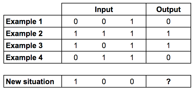
Training data: Only the first column of input impacts the output

Since the code has been written in a previous version of Python, here are also included fully functional updated version for Python 3.6. Here is the light 9-line initial code for the single layer neural network.

Training Process

1. Take inputs, adjust with weights (positive or negative numbers), norm them through a sigmoid function
2. Calculate the error between the neuron’s output and the actual training data set
3. Adjust weights according to the error
4. Repeat 10,000 times

Calculate the neuron’s output

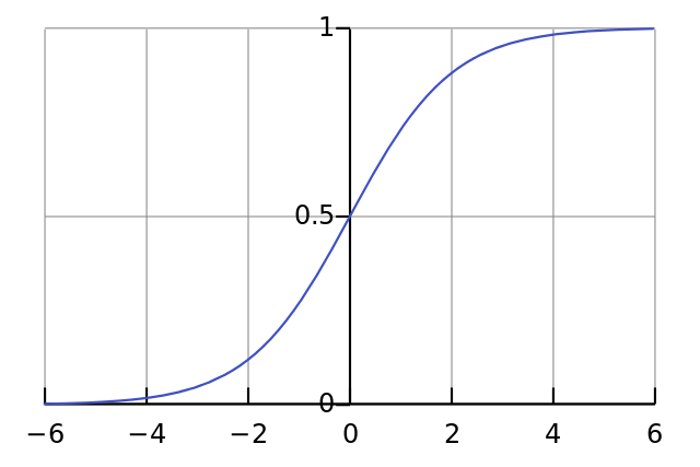
Sum the weighted input data into a sigmoid function to obtain normed results in the interval ]0;1[

The final formula for the output of the neuron is:

Adjusting weights

Use the error weighted derivative = gradient descent

1. The neuron output from the sigmoid function indicates that if the output is close to 0 or 1, the data was close to the expected result
2. Close to 0 or 1, the derivative of the sigmoid function is almost flat
3. The adjustment to the weights based upon the derivative from the sigmoid function will therefore be very small when the neuron’s output is close to expected results or large when results differ from expectations

The sigmoid derivative equation is:

So the final equation to adjust weights is:

Here is a fully functional version of the final code for the single-layer neural network with all details and comments, updated for Python 3.6.

Multiple-layer neural net

In the second post, the building of a multiple neural network is detailed through the following key steps reproduced. Bear in mind that such a neural network may be to complicated to solve simple problems and that it is best to understand nonlinear patterns, where the second layer of neurons can take combination of data inputs into account.

Here this two-layer neural net is used to understand how two columns in the data influence the results.

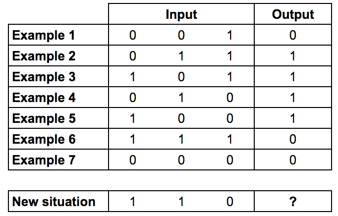
Training data: The two first columns of input impact the output (XOR gate)

As Milo Spencer-Harper reminds us in his article, multiple layers are the source of the revolution in machine learning and artificial intelligence:

The process of adding more layers to a neural network, so it can think about combinations, is called deep learning.

The main difference in the code from the single-layer neural net is that the two layers influence the calculations for the error, and therefore the adjustment of weights. The errors from the second layer of neurons need to be propagated backwards to the first layer, this is called backpropagation.

Here is a fully functional version of the code for a two-layer neural network with all details and comments, updated for Python 3.6.

To sum up, in the following video, Siraj Raval goes over the detailed programming of a similar neural net (the original from Andrew Trask) in 4 minutes.

Attention: he uses an older version of Python, he also builds a 3-layer neural net, but the first layer is actually the input data without computation.